Hi! Welcome back to the second part of my series on different machine learning model evaluation metrics. In the previous post I’ve talked about some essential metrics that can be applied to a binary classification problem.

In this post, let’s see how some of them can be extended to a multi-class case:

• What does confusion matrix look like for a multi-class problem?
• How are micro-, macro- and weighted-averaged metrics calculated?
• Log Loss for multi-class problem

Confusion Matrix

Just like you generate a confusion matrix for a binary problem, you can generate one for a multi-class problem. For an example, I’ll take a toy dataset from sklearn.datasets with hand-written digits. This dataset contains images of hand-written digits: 10 classes where each class refers to a digit, and after training a LogisticRegression or some other model on it, I can call confusion_matrix from sklearn.metrics and pass to it the test data: true values first, then predictions. The resulting array would look something like this:

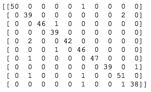
As with the binary case, the rows represent the true labels, and the columns show the predicted labels. Both rows and columns are sorted by label, so the first row shows all the samples that have a true label 0, and the last row show all the samples that have a true label 9. Of course, it’s quite hard to interpret this matrix in this raw format. So typically you’d want to plot it as a heatmap. You can find an example of how to plot a confusion matrix in scikit-learn docs, it’s not too tricky.

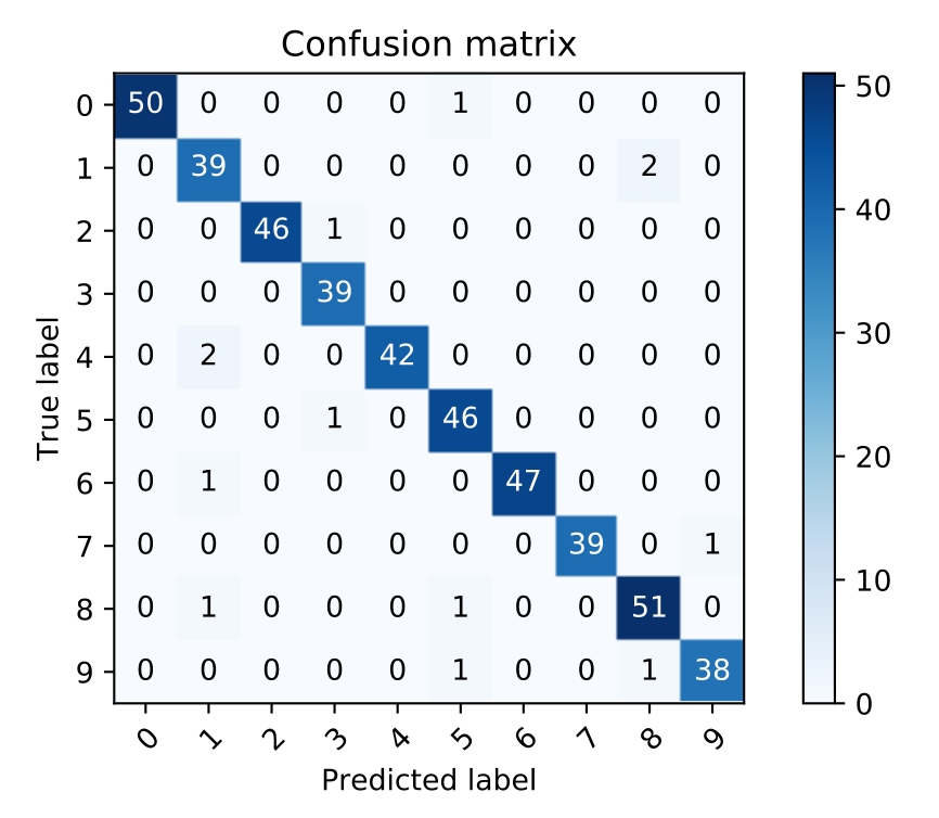
Now, you can already diagnose what sort of errors a model is making. For instance, here we can see that the model predicted 8 when the actual label was 1 two times, and predicted 1 when the label was 4 another couple of times, and so on. Like in the binary case, the diagonal of the matrix represents all the times the model prediction was correct.

However now we don’t really have the notion of true negatives, false positives and so on. Nonetheless, there’s a way to use such metrics as Precision, Recall and F1 score.

For these metrics to be calculated on a multi-class problem, the problem needs to be treated as a set of binary problems (“one-vs-all”). In this case a metric, for instance, Precision can be calculated per class, and then the final metric will be the average of the per-class metrics. Of course, there’s more than one way to average, and it does make a difference.

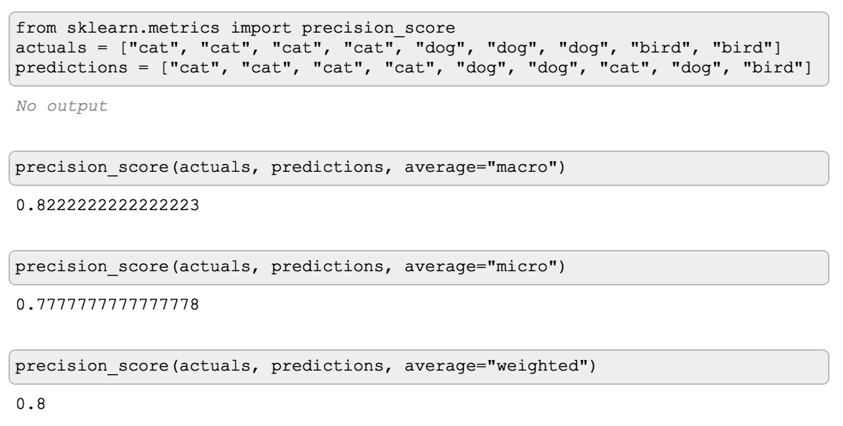
Here, the precision_score is calculated three times, each time with a different average parameter: micro, macro and weighted. Let’s see what’s the difference in how they’re calculated.

Micro-, Macro-, Weighted-averaged Precision

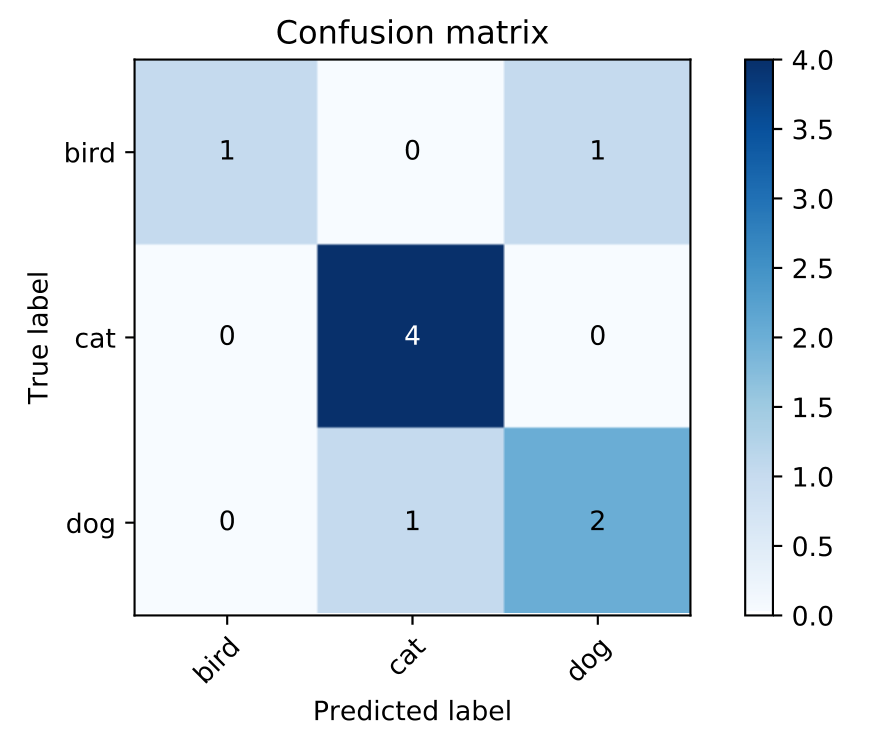
Let’s take the previous example, and draw the true values and the predictions as a table:

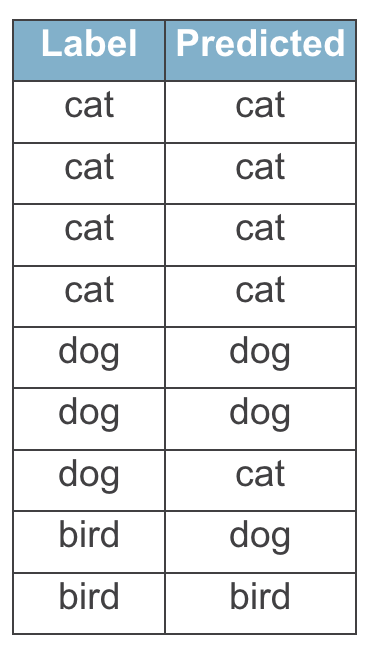
From this small table you can easily imagine what a confusion matrix would look like:

Next thing, for each class we need to figure out what would be the True Positives, False Positives and False Negatives, if we treat it as “one-vs-all” problem. Technically, we don’t need False Negatives to calculate Precision, but we would need it for Recall and F1 score, so let’s keep it.

Here’s what it would look like for a class “bird”":

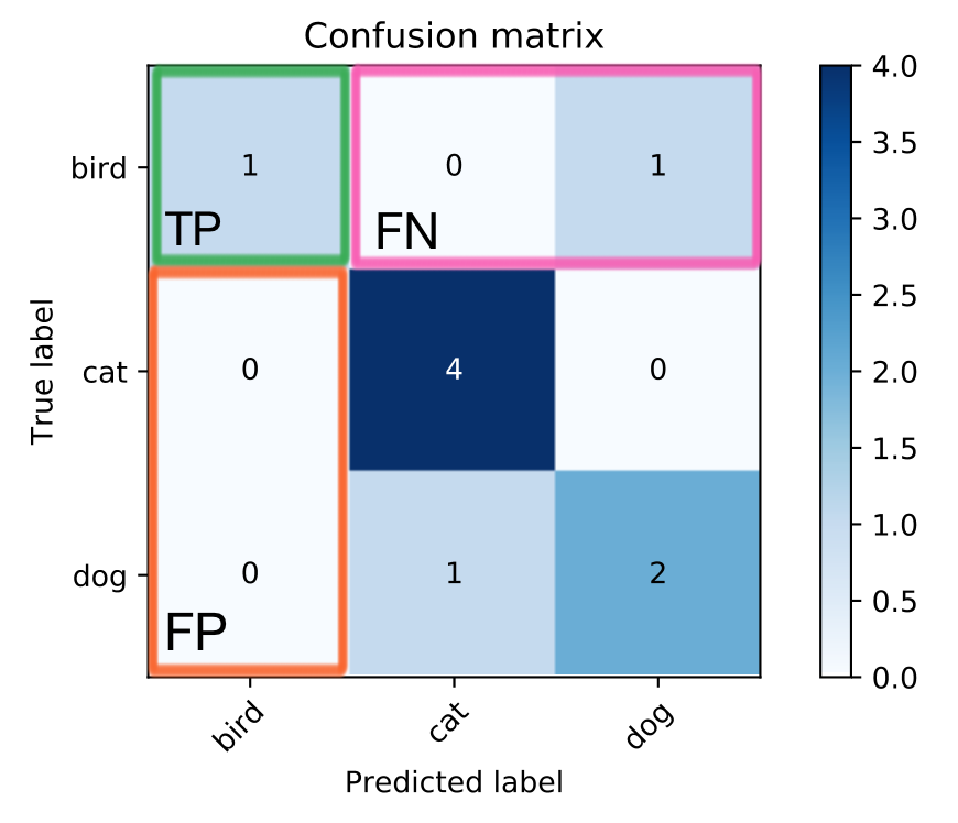
• True Positives: We only have one cell (highlighted green) where the true label was “bird” and the predicted label was “bird”. The number in that cell will be the True Positives.
• False Positives: These are all those cases where “bird” was predicted, but the actual label was something else. These are all the cells in the same column as the true positives except the cell with the TP (highlighted orange). So, False Positives are the sum of the values in the orange area.
• False Negatives: These are all the times where the actual label was “bird” but the model predicted something else. These are all the cells in the same row as the true positives (highlighted pink) except the cell with TP. False Negatives is the sum of all those cells.

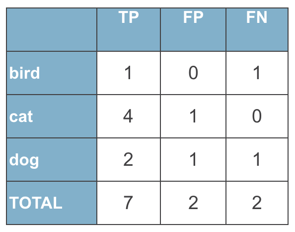
By doing the same for all the classes, we can write down these numbers into a table, and sum them up into totals:

Next thing, we can calculate presision for each class:

$$Precision_{birds} = \frac{TP_{birds}}{TP_{birds} + FP_{birds}} = \frac{1}{1 + 0} = 1$$

$$Precision_{cats} = \frac{TP_{cats}}{TP_{cats} + FP_{cats}} = \frac{4}{4 + 1} = 0.8$$

$$Precision_{dogs} = \frac{TP_{dogs}}{TP_{dogs} + FP_{dogs}} = \frac{2}{2 + 1} = 0.667$$

Let’s add these numbers to the table, and add a column that notes how many samples of each class we had:

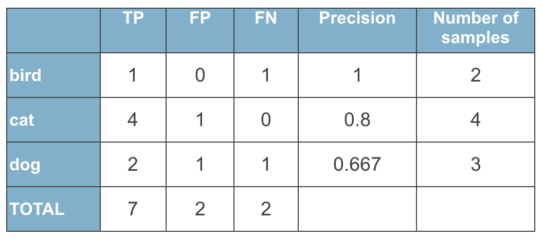
Once we have this table, it’s very easy to calculate precision with different averaging strategies.

Micro-averaged Precision is calculated as precision of Total values:

$$\text{Micro-averaged Precision} = \frac{TP_{total}}{TP_{total} + FP_{total}} = \frac {7}{7+2} = 0.7777$$

Macro-averaged Precision is calculated as an average of Precisions of all classes:

$$\text{Macro-averaged Precision} = \frac{1}{3}{Precision_{birds} + Precision_{cats} + Precision_{dogs}} = \frac {1}{3}(1+0.8+0.6666)=0.8222$$

Weighted-averaged Precision is also calculated based on Precision per class but takes into account the number of samples of each class in the data:

$$\text{Weighted-averaged Precision} = \frac{Precision_{birds}*N_{birds} + Precision_{cats}*N_{birds}+Precision_{dogs}*N_{birds}}{\text{Total number of samples}} = \frac {1*2 + 0.8*4+0.6666*3}{2+4+3} = 0.8$$

Now that you know how it’s calculated, it’s easy to see that in:

• Micro-averaged: all samples equally contribute to the final averaged metric
• Macro-averaged: all classes equally contribute to the final averaged metric
• Weighted-averaged: each classes’s contribution to the average is weighted by its size

So which type of averaging is preferable? As usual, this largely depends on the problem you’re trying to solve. Do you have a class-imbalanced dataset? Is one class more important to get right than others? If you have an under-represented class which is important to your problem, macro-averaging may better, as it will highlight the performance of a model on all classes equally. On the other hand, if the assumption that all classes are equally important is not true, macro-averaging will over-emphasize the low performance on an infrequent class. Micro-averaging may be preferred in multilabel settings, including multiclass classification where a majority class is to be ignored.
There’s also a “samples” averaging strategy that applies only to multi-label problems. You can read more about it in the scikit-learn documentation.

Multi-class Log Loss

Multiclass-log loss is no different than log loss for the binary problem which I talked about in the previous post. In fact, log loss for the binary problem is simply a special case of it.

In more general case, the formula for log loss will look like this:

$$- \frac{1}{N} \sum_{i=1}^N \sum_{j=1}^M y_{ij} \log , p_{ij}$$

where $N$ is the number of samples, $M$ is the number of labels, $y_{ij}$ is a binary indicator whether a label $j$ is the correct label for the samples $i$, and $p_{ij}$ is the model’s output probability of label $j$ being the correct label for the samples $i$.

If the formula is too much to handle, I find it easier to think of it as of a for cycle like this one:

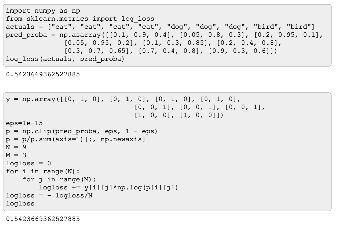
Now, of course, if you look in how it’s calculated in scikit-learn, you won’t find for cycles, because vectorized operations are much faster. But to me, “spelling out” a formula like this sometimes helps for it to “click” for me.

Thanks for reading! Check out more posts about evaluation metrics:

• Part 1: binary classification metrics
• Part 3: regression metrics