In the final part of my series on ML model evaluation metrics we’ll talk about metrics that can be applied to regression problems. If you’d like to read about evaluation metrics for classification problems, check out my other blog posts: part 1: binary classification and part 2: multi-class classification.

Here’s what’s on the today’s menu:

• R squared
• MAE
• MSE
• RMSE
• MAE vs RMSE as an evaluation metric
• RMSLE

In this post you’re going to see some more formulas, but I personally find that despite that, the evaluation metrics for regression tasks are a conceptually simpler. For instance, we don’t have to deal with the output probabilities. We’re dealing with a continuous value as a target, and the model predicts a continuous value. When we subtract one from the other, we get our model’s error, or more correctly this is called a residual. Now, the question is: how do we describe the overall model performance based on individual residuals? There’s a few ways of going about it.

R squared

If you remember from my previous posts, each classifier in scikit-learn has a score method that will return your model’s classification accuracy. This is sort of a default evaluation metric for a classifier. Regressors have a score method too, and for them the score method returns R squared which is also called coefficient of determination:

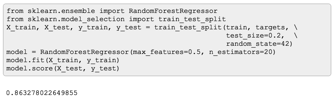
This is a metric that indicates how well model predictions approximate the true values, where 1 indicates perfect fit, and 0 would be R squared of a DummyRegressor that always predicts the mean of the data. Here’s how it’s calculated:

$$R^2(y, \hat{y}) = 1 - \frac{\sum_{i=1}^n (y_i - \hat{y}_i)^2}{\sum_{i=1}^{n} (y_i - \bar{y})^2}$$

where $y$ is the actual value, $\hat{y}$ is the predicted value, and $\bar{y}$ is the mean of the actual values.

In the numerator here we calculate the residuals for each sample, square them and sum them up. In the denominator we calculate for each sample, the distance between the actual value and the mean of all values.

So if our model is always predicting the mean (a DummyRegressor) the numerator will be equal to the denominator, and R squared will be equal to $1 - 1 = 0$. So R squared is showing how much better a model is performing compared to a dummy.

Of course, technically, R squared can be negative - say, the model is always predicting an infinitely large number, but if you’re getting a negative R squared, this means something is seriously wrong either with the model, or, perhaps, with the data.

One great thing about R squared is that it has an intuitive scale that does not depend on the units of the target variable. It doesn’t matter if you’re predicting prices, distance, weight or something else. However it also says nothing about the prediction error of the model, which is quite important in most cases. That’s why typically you’d want to compliment R squared with a metric that helps you understand the error as well. Let’s look at some metrics that help with that.

MAE

One of such metrics is Mean Absolute Error(MAE). It is quite straightforward. For each sample, we calculate the difference between the actual value and the predicted value (residual) and take an absolute value of that. Next, we simply get the average of all those absolute values:

$$\text{MAE}(y, \hat{y}) = \frac{1}{n} \sum_{i=1}^{n} \left| y_i - \hat{y}_i \right|$$

If formulas are not your cup of tea, here’s how you can express the same thing in python:

In scikit-learn, you can get this metric from sklearn.metrics:

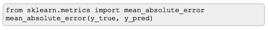
The reason why we take the absolute value of every residual before calculating the average is so that the positive and negative residuals don’t cancel each other out.

MSE

If instead of taking absolute values of residuals we’ll square them, we’ll get Mean Squared Error(MSE):

$$\text{MSE}(y, \hat{y}) = \frac{1}{n} \sum_{i=1}^{n} (y_i - \hat{y}_i)^2$$

Same in python:

With scikit-learn:

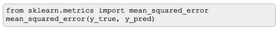
Just like with the MAE, negative and positive residuals won’t cancel each other out, but in this case the metric no longer has the same units as the target value. The error is now expressed in squared target units.

RMSE

Finally, if we take a square root of MSE, we’ll get a metric called Root Mean Squared Error(RMSE). This metric, again has the same units as the target values.

$$\text{RMSE}(y, \hat{y}) = \sqrt{\frac{1}{n} \sum_{i=1}^{n} (y_i - \hat{y}_i)^2}$$

Same in python:

With scikit-learn:

RMSE is commonly used as both an evaluation metric, and a loss function. This is because unlike Mean Absolute Error, RMSE is smoothly differentiable, so it makes sense to use it as a loss function. Having the same evaluation metric as a loss function can have its benefits - this is something the model has already optimized for. But every now and then you can see people preferring MAE to RMSE. Let’s see what these two metrics have in common, and what is different.

MAE vs RMSE

Let’s start by looking at what these two metrics have in common.

• First, both MAE and RMSE can range from 0 to ∞.
• MAE and RMSE have the same units as the target values
• They are indifferent to the direction of the errors (we’re either taking an absolute value or squaring each residual)
• The lower the metric value, the better

Now, how are MAE and RMSE different?

• RMSE gives a relatively high weight to large errors due to the fact that the residual is squared before averaging
• On the other hand, averaging absolute values makes MAE more robust to outliers
• RMSE is differentiable (which is correct, but not really important for an evaluation metric)

You can find a good number of articles arguing that for evaluating a regression model’s performance MAE is a more appropriate metric than RMSE. Most of the arguments for this are likely to be based on the paper from 2005 called “Advantages of the mean absolute error (MAE) over the root mean square error (RMSE) in assessing average model performance” by Cort J. Willmott and Kenji Matsuura. The authors state that “the RMSE … is an inappropriate and misinterpreted measure of average error.”, and that “dimensioned evaluations and inter-comparisons of average model-performance error, therefore, should be based on MAE.”

However, a later paper from 2009 called “Root mean square error (RMSE) or mean absolute error (MAE)?" by Tianfeng Chai and R. R. Draxler, disagrees with the previous paper. The authors conclude that “The RMSE is more appropriate to represent model performance than the MAE when the error distribution is expected to be Gaussian.”

For most practical purposes, I find that RMSE is a good choice for an evaluation metric, and MAE can be useful in those cases when it is important to downplay the outliers.

RMSLE

There’s a variation of RMSE that is sometimes more convenient to use - Root Mean Squared Logarithmic Error (RMSLE). The only difference from the RMSE is that instead of using y values directly, it uses logarithm of them:

$$\text{RMSLE}(y, \hat{y}) = \sqrt{\frac{1}{n} \sum_{i=1}^{n} (\log_e (y_i + 1) - \log_e (\hat{y}_i + 1) )^2}$$

Note: the constant 1 is added in the logarithm is simply because log of 0 is not defined.

With scikit-learn:

What taking a log here gives us is a measure or relative error. This metric is best to use when targets are having exponential growth, such as population counts, average sales of a commodity over a span of years etc. This metric allows to take the scale of the values into account, e.g. the error of 5 dollars in a 50 dollars purchase is a significant error, whereas the same error of 5 dollars in a 500 000 dollars purchase is much less important.

An interesting side-effect of this metric to keep in mind is that this metric penalizes an under-predicted estimate greater than an over-predicted estimate.

I hope this will help you find the right metric for your next machine learning problem, or to understand why one metric have been chosen in a given task or competition. Thanks for reading!

Check out more posts about evaluation metrics:

Experiments with links:

• Part 1: binary classification metrics and
• Part 2: multi-class classification.